Download this notebook from github.

Uncertainty partitioning

Here we estimate the sources of uncertainty for an ensemble of climate model projections. The data is the same as used in the IPCC WGI AR6 Atlas.

Fetch data

We’ll only fetch a small sample of the full ensemble to illustrate the logic and data structure expected by the partitioning algorithm.

from __future__ import annotations

import matplotlib as mpl
import numpy as np
import pandas as pd
import xarray as xr
from matplotlib import pyplot as plt

import xclim.ensembles

# The directory in the Atlas repo where the data is stored
# host = "https://github.com/IPCC-WG1/Atlas/raw/main/datasets-aggregated-regionally/data/CMIP6/CMIP6_tas_land/"
host = "https://raw.githubusercontent.com/IPCC-WG1/Atlas/main/datasets-aggregated-regionally/data/CMIP6/CMIP6_tas_land/"

# The file pattern, e.g. CMIP6_ACCESS-CM2_ssp245_r1i1p1f1.csv
pat = "CMIP6_{model}_{scenario}_{member}.csv"

# Here we'll download data only for a very small demo sample of models and scenarios.

# Download data for a few models and scenarios.
models = ["ACCESS-CM2", "CMCC-CM2-SR5", "CanESM5"]

# The variant label is not always r1i1p1f1, so we need to match it to the model.
members = ["r1i1p1f1", "r1i1p1f1", "r1i1p1f1"]

# GHG concentrations and land-use scenarios
scenarios = ["ssp245", "ssp370", "ssp585"]

data = []
for model, member in zip(models, members):
    for scenario in scenarios:
        url = host + pat.format(model=model, scenario=scenario, member=member)

        # Fetch data using pandas
        df = pd.read_csv(url, index_col=0, comment="#", parse_dates=True)["world"]
        # Convert to a DataArray, complete with coordinates.
        da = (
            xr.DataArray(df)
            .expand_dims(model=[model], scenario=[scenario])
            .rename(date="time")
        )
        data.append(da)

Create an ensemble

Here we combine the different models and scenarios into a single DataArray with dimensions model and scenario. Note that the names of those dimensions are important for the uncertainty partitioning algorithm to work.

Note that the xscen library provides a helper function xscen.ensembles.build_partition_data to build partition ensembles.

# Combine DataArrays from the different models and scenarios into one.
ens_mon = xr.combine_by_coords(data)["world"]

# Then resample the monthly time series at the annual frequency
ens = ens_mon.resample(time="Y").mean()
ssp_col = {
    "ssp126": "#1d3354",
    "ssp245": "#eadd3d",
    "ssp370": "#f21111",
    "ssp585": "#840b22",
}
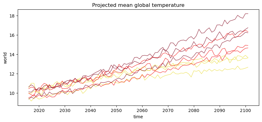
plt.figure(figsize=(10, 4))
for scenario in ens.scenario:
    for model in ens.model:
        ens.sel(scenario=scenario, model=model).plot(
            color=ssp_col[str(scenario.data)], alpha=0.8, lw=1
        )
plt.title("Projected mean global temperature");

/home/docs/checkouts/readthedocs.org/user_builds/xclim/conda/stable/lib/python3.12/site-packages/xarray/core/groupby.py:532: FutureWarning: 'Y' is deprecated and will be removed in a future version, please use 'YE' instead.
  index_grouper = pd.Grouper(

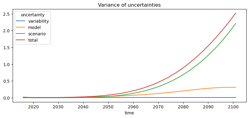
Now we’re able to partition the uncertainties between scenario, model, and variability using the approach from Hawkins and Sutton.

By default, the function uses the 1971-2000 period to compute the baseline. Since we haven’t downloaded historical simulations, here we’ll just use the beginning of the future simulations.

mean, uncertainties = xclim.ensembles.hawkins_sutton(ens, baseline=("2016", "2030"))
plt.figure(figsize=(10, 4))
uncertainties.plot(hue="uncertainty")
plt.title("Variance of uncertainties");

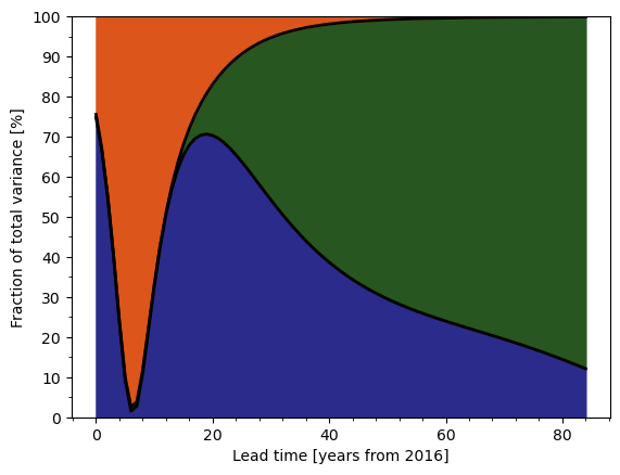
From there, it’s relatively straightforward to compute the relative strength of uncertainties, and create graphics similar to those found in scientific papers.

Note that the figanos library provides a function fg.partition to plot the graph below.

colors = {
    "variability": "#DC551A",
    "model": "#2B2B8B",
    "scenario": "#275620",
    "total": "k",
}
names = {"variability": "Internal variability"}


def graph_fraction_of_total_variance(variance, ref="2000", ax=None):
    """Figure from Hawkins and Sutton (2009) showing fraction of total variance.

    Parameters
    ----------
    variance: xr.DataArray
      Variance over time of the different sources of uncertainty.
    ref: str
      Reference year. Defines year 0.
    ax: mpl.axes.Axes
      Axes in which to draw.

    Returns
    -------
    mpl.axes.Axes
    """
    if ax is None:
        fig, ax = plt.subplots(1, 1)

    # Compute fraction
    da = variance / variance.sel(uncertainty="total") * 100

    # Select data from reference year onward
    da = da.sel(time=slice(ref, None))

    # Lead time coordinate
    lead_time = add_lead_time_coord(da, ref)

    # Draw areas
    y1 = da.sel(uncertainty="model")
    y2 = da.sel(uncertainty="scenario") + y1
    ax.fill_between(lead_time, 0, y1, color=colors["model"])
    ax.fill_between(lead_time, y1, y2, color=colors["scenario"])
    ax.fill_between(lead_time, y2, 100, color=colors["variability"])

    # Draw black lines
    ax.plot(lead_time, np.array([y1, y2]).T, color="k", lw=2)

    ax.xaxis.set_major_locator(mpl.ticker.MultipleLocator(20))
    ax.xaxis.set_minor_locator(mpl.ticker.AutoMinorLocator(n=5))

    ax.yaxis.set_major_locator(mpl.ticker.MultipleLocator(10))
    ax.yaxis.set_minor_locator(mpl.ticker.AutoMinorLocator(n=2))

    ax.set_xlabel(f"Lead time [years from {ref}]")
    ax.set_ylabel("Fraction of total variance [%]")

    ax.set_ylim(0, 100)

    return ax


def add_lead_time_coord(da, ref):
    """Add a lead time coordinate to the data. Modifies da in-place."""
    lead_time = da.time.dt.year - int(ref)
    da["Lead time"] = lead_time
    da["Lead time"].attrs["units"] = f"years from {ref}"
    return lead_time

graph_fraction_of_total_variance(uncertainties, ref="2016");