Spatial Analogues examples

xclim provides the xclim.analog module that allows the finding of spatial analogues.

Spatial analogues are maps showing which areas have a present-day climate that is analogous to the future climate of a given place. This type of map can be useful for climate adaptation to see how well regions are coping today under specific climate conditions. For example, officials from a city located in a temperate region that may be expecting more heatwaves in the future can learn from the experience of another city where heatwaves are a common occurrence, leading to more proactive intervention plans to better deal with new climate conditions.

Spatial analogues are estimated by comparing the distribution of climate indices computed at the target location over the future period with the distribution of the same climate indices computed over a reference period for multiple candidate regions.

[1]:

from __future__ import annotations

import matplotlib.pyplot as plt

from xclim import analog
from xclim.core.calendar import convert_calendar
from xclim.testing import open_dataset

Input data

The “target” input of the computation is a collection of indices over a given location and for a given time period. Here we have three indices computed on bias-adjusted daily simulation data from the CanESM2 model, as made available through the CMIP5 project. We chose to look at the climate of Chibougamau, a small city in northern Québec, for the 2041-2070 period.

[2]:

sim = open_dataset(
    "SpatialAnalogs/CanESM2_ScenGen_Chibougamau_2041-2070.nc",
    decode_timedelta=False,
)
sim

The goal is to find regions where the present climate is similar to that of a simulated future climate. We call “candidates” the dataset that contains the present-day indices. Here we use gridded observations provided by Natural Resources Canada (NRCan). This is the same data that was used as a reference for the bias-adjustment of the target simulation, which is essential to ensure the comparison holds.

A good test to see if the data is appropriate for computing spatial analog is the so-called “self-analog” test. It consists in computing the analogs using the same time period on both the target and the candidates. The test passes if the best analog is the same point as the target. Some authors have found that in some cases, a second bias-adjustment over the indices is needed to ensure that the data passes this test (see Grenier et al. (2019)). However, in this introductory notebook, we can’t run this test and will simply assume the data is coherent.

[3]:

obs = open_dataset(
    "SpatialAnalogs/NRCAN_SECan_1981-2010.nc",
    decode_timedelta=False,
)
obs

[4]:

obs.tg_mean.isel(time=0).plot()
plt.plot(sim.lon, sim.lat, "ro");  # Plot a point over Chibougamau

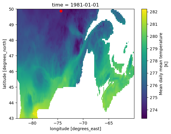
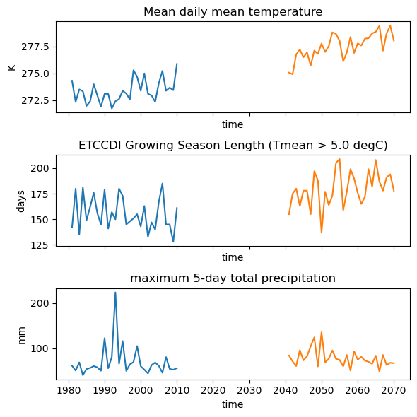
Let’s plot the timeseries over Chibougamau for both periods to get an idea of the climate change between these two periods. For the purpose of the plot, we’ll need to convert the calendar of the data as the simulation uses a noleap calendar.

[5]:

fig, axs = plt.subplots(nrows=3, figsize=(6, 6), sharex=True)
sim_std = convert_calendar(sim, "default")
obs_chibou = obs.sel(lat=sim.lat, lon=sim.lon, method="nearest")

for ax, var in zip(axs, obs_chibou.data_vars.keys()):
    obs_chibou[var].plot(ax=ax, label="Observation")
    sim_std[var].plot(ax=ax, label="Simulation")
    ax.set_title(obs_chibou[var].long_name)
    ax.set_ylabel(obs_chibou[var].units)
fig.tight_layout()

All the work is encapsulated in the xclim.analog.spatial_analogs function. By default, the function expects that the distribution to be analysed is along the “time” dimension, like in our case. Inputs are datasets of indices, the target and the candidates should have the same indices and at least the time variable in common. Normal xarray broadcasting rules apply for the other dimensions.

There are many metrics available to compute the dissimilarity between the indicator distributions. For our first test, we’ll use the mean annual temperature (tg_mean) and the simple standardized Euclidean distance metric (seuclidean). This is a very basic metric that only computes the distance between the means. All algorithms used to compare distributions are available through the xclim.analog.spatial_analogs function. They also live as well-documented functions in the same module or in the xclim.analog.metrics dictionary.

[6]:

results = analog.spatial_analogs(
    sim[["tg_mean"]], obs[["tg_mean"]], method="seuclidean"
)

results.plot()
plt.plot(sim.lon, sim.lat, "ro", label="Target")


def plot_best_analog(scores, ax=None):
    scores1d = scores.stack(site=["lon", "lat"])
    lon, lat = scores1d.isel(site=scores1d.argmin("site")).site.item()
    ax = ax or plt.gca()
    ax.plot(lon, lat, "r*", label="Best analog")


plot_best_analog(results)
plt.title("Average temperature - Standardized Euclidean distance")
plt.legend();

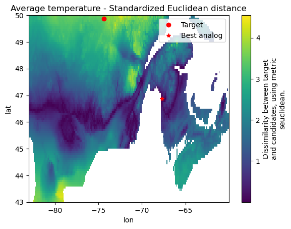
This shows that the average temperature projected by our simulation for Chibougamau in 2041-2070 will be similar to the 1981-2010 average temperature of a region approximately extending zonally between 46°N and 47°N. Evidently, this metric is limited as it only compares the time averages. Let’s run this again with the “Zech-Aslan” metric, one that compares the whole distribution.

[7]:

results = analog.spatial_analogs(
    sim[["tg_mean"]], obs[["tg_mean"]], method="zech_aslan"
)

results.plot(center=False)
plt.plot(sim.lon, sim.lat, "ro", label="Target")
plot_best_analog(results)
plt.title('Average temperature - Zech-Aslan "energy" metric')
plt.legend();

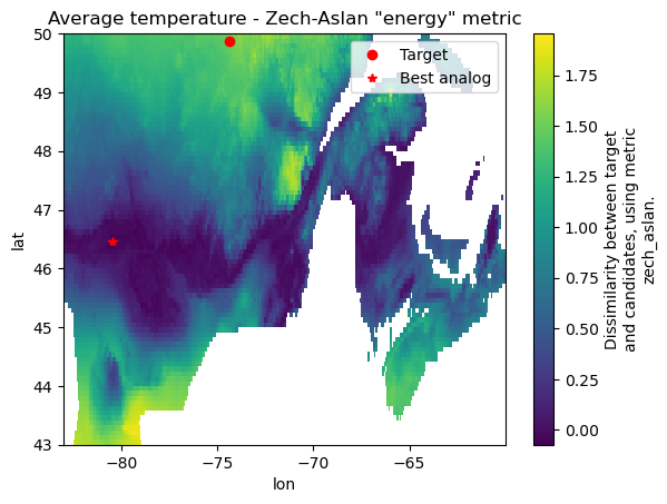
The new map is quite similar to the previous one, but notice how the scale has changed. Each metric defines its own scale (see the docstrings), but in all cases, lower values imply fewer differences between distributions. Notice also how the best analog has moved. This illustrates a common issue with these computations : there’s a lot of noise in the results, and the absolute minimum may be extremely sensitive and move all over the place.

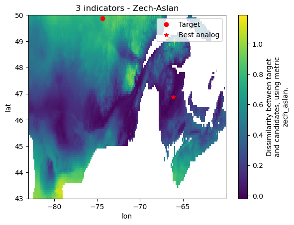
These univariate analogies are interesting, but the real power of this method is that it can perform multivariate analyses.

[8]:

results = analog.spatial_analogs(sim, obs, method="zech_aslan")

results.plot(center=False)
plt.plot(sim.lon, sim.lat, "ro", label="Target")
plot_best_analog(results)
plt.legend()
plt.title("3 indicators - Zech-Aslan");

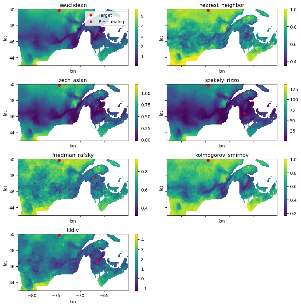
As said just above, results depend on the metric used. For example, some of the metrics include some sort of standardization, while others don’t. In the latter case, this means the absolute magnitude of the indices influences the results, i.e. analogies depend on the units. This information is written in the docstring.

Some are also much more efficient than other (for example : seuclidean or zech_aslan, compared to kolmogorov_smirnov or friedman_rafsky).

[9]:

# This cell is slow.
import time

fig, axs = plt.subplots(4, 2, sharex=True, sharey=True, figsize=(10, 10))
for metric, ax in zip(analog.metrics.keys(), axs.flatten()):
    start = time.perf_counter()
    results = analog.spatial_analogs(sim, obs, method=metric)
    print(f"Metric {metric} took {time.perf_counter() - start:.0f} s.")

    results.plot(center=False, ax=ax, cbar_kwargs={"label": ""})
    ax.plot(sim.lon, sim.lat, "ro", label="Target")
    plot_best_analog(results, ax=ax)
    ax.set_title(metric)
axs[0, 0].legend()
axs[-1, -1].set_visible(False)
fig.tight_layout()

Metric seuclidean took 2 s.
Metric nearest_neighbor took 8 s.
Metric zech_aslan took 3 s.
Metric szekely_rizzo took 2 s.
Metric friedman_rafsky took 24 s.
Metric kolmogorov_smirnov took 9 s.
Metric kldiv took 12 s.