Download this notebook from github.

Workflow Examples

xclim is built on very powerful multiprocessing and distributed computation libraries, notably xarray and dask.

xarray is a python package making it easy to work with n-dimensional arrays. It labels axes with their names [time, lat, lon, level] instead of indices [0,1,2,3], reducing the likelihood of bugs and making the code easier to understand. One of the key strengths of xarray is that it knows how to deal with non-standard calendars (we’re looking at you, “360_days”) and can easily resample daily time series to weekly, monthly, seasonal or annual periods. Finally, xarray is tightly integrated with dask, a package that can automatically parallelize operations.

The following are a few examples to consult when using xclim to subset NetCDF arrays and compute climate indicators, taking advantage of the parallel processing capabilities offered by xarray and dask. For more information about these projects, please see their documentation pages:

• xarray documentation

• dask documentation

Environment configuration

from __future__ import annotations

# File handling libraries
import tempfile
from pathlib import Path

import xarray as xr

# Set xarray to use HTML for displaying outputs
xr.set_options(display_style="html")

import xclim.indices

# Output folder
output_folder = Path(tempfile.mkdtemp())

Setting up the Dask client: parallel processing

In this example, we are using the **dask.distributed** submodule. This is not installed by default in a basic xclim installation. Be sure to add distributed to your Python installation before setting up parallel processing operations!

First, we create a pool of workers that will wait for jobs. The xarray library will automatically connect to these workers and dispatch them jobs that can be run in parallel.

The dashboard link lets you see in real time how busy those workers are.

• dask distributed documentation

This step is not mandatory, as dask will fall back to its “single machine scheduler” if a Client is not created. However, this default scheduler doesn’t allow you to set the number of threads or a memory limit and doesn’t start the dashboard, which can be quite useful to understand your task’s progress.

from distributed import Client

# Depending on your workstation specifications, you may need to adjust these values.
# On a single machine, n_workers=1 is usually better.
client = Client(n_workers=1, threads_per_worker=4, memory_limit="4GB")
client

Client

Client-b2f17bd1-d597-11ee-9875-0242ac110002

Connection method: Cluster object	Cluster type: distributed.LocalCluster
Dashboard: http://127.0.0.1:8787/status

Cluster Info

LocalCluster

9b8c4941

Dashboard: http://127.0.0.1:8787/status	Workers: 1
Total threads: 4	Total memory: 3.73 GiB
Status: running	Using processes: True

Scheduler Info

Scheduler

Scheduler-b69fb0ef-146d-4cbc-bd5b-cca3c58c3e57

Comm: tcp://127.0.0.1:36047	Workers: 1
Dashboard: http://127.0.0.1:8787/status	Total threads: 4
Started: Just now	Total memory: 3.73 GiB

Workers

Worker: 0

Comm: tcp://127.0.0.1:42379	Total threads: 4
Dashboard: http://127.0.0.1:40399/status	Memory: 3.73 GiB
Nanny: tcp://127.0.0.1:33409
Local directory: /tmp/dask-scratch-space/worker-np0r8adv

Creating xarray datasets

To open a NetCDF file with xarray, we use xr.open_dataset(<path to file>). By default, the entire file is stored in one chunk, so there is no parallelism. To trigger parallel computations, we need to explicitly specify the chunk size.

In this example, instead of opening a local file, we pass an OPeNDAP URL to xarray. It retrieves the data automatically. Notice also that opening the dataset is quite fast. In fact, the data itself has not been downloaded yet, only the coordinates and the metadata. The downloads will be triggered only when the values need to be accessed directly.

dask’s parallelism is based on memory chunks; We need to tell xarray to split our NetCDF array into chunks of a given size, and operations on each chunk of the array will automatically be dispatched to the workers.

data_url = "https://pavics.ouranos.ca/twitcher/ows/proxy/thredds/dodsC/datasets/simulations/bias_adjusted/cmip5/ouranos/cb-oura-1.0/day_ACCESS1-3_historical+rcp85_r1i1p1_na10kgrid_qm-moving-50bins-detrend_1950-2100.ncml"

# Chunking in memory along the time dimension.
# Note that the data type is a 'dask.array'. xarray will automatically use client workers.
ds = xr.open_dataset(
    data_url,
    chunks={"time": 365, "lat": 168, "lon": 150},
    drop_variables=["ts", "time_vectors"],
)
print(ds)

<xarray.Dataset> Size: 169GB
Dimensions:  (lat: 320, lon: 797, time: 55152)
Coordinates:
  * lat      (lat) float32 1kB 66.62 66.54 66.46 66.37 ... 40.21 40.12 40.04
  * lon      (lon) float32 3kB -120.8 -120.7 -120.6 ... -54.63 -54.55 -54.46
  * time     (time) datetime64[ns] 441kB 1950-01-01 1950-01-02 ... 2100-12-31
Data variables:
    tasmin   (time, lat, lon) float32 56GB dask.array<chunksize=(365, 168, 150), meta=np.ndarray>
    tasmax   (time, lat, lon) float32 56GB dask.array<chunksize=(365, 168, 150), meta=np.ndarray>
    pr       (time, lat, lon) float32 56GB dask.array<chunksize=(365, 168, 150), meta=np.ndarray>
Attributes: (12/26)
    Conventions:                CF-1.5
    title:                      Ouranos standard ensemble of bias-adjusted cl...
    history:                    CMIP5 compliant file produced from raw ACCESS...
    institution:                Ouranos Consortium on Regional Climatology an...
    source:                     ACCESS1-3 2011. Atmosphere: AGCM v1.0 (N96 gr...
    driving_experiment:         historical,rcp85
    ...                         ...
    frequency:                  day
    modeling_realm:             atmos
    target_dataset:             CANADA : ANUSPLIN interpolated Canada daily 3...
    target_dataset_references:  CANADA : https://doi.org/10.1175/2011BAMS3132...
    driving_institution:        Commonwealth Scientific and Industrial Resear...
    driving_institute_id:       CSIRO-BOM

print(ds.tasmin.chunks)

((365, 365, 365, 365, 365, 365, 365, 365, 365, 365, 365, 365, 365, 365, 365, 365, 365, 365, 365, 365, 365, 365, 365, 365, 365, 365, 365, 365, 365, 365, 365, 365, 365, 365, 365, 365, 365, 365, 365, 365, 365, 365, 365, 365, 365, 365, 365, 365, 365, 365, 365, 365, 365, 365, 365, 365, 365, 365, 365, 365, 365, 365, 365, 365, 365, 365, 365, 365, 365, 365, 365, 365, 365, 365, 365, 365, 365, 365, 365, 365, 365, 365, 365, 365, 365, 365, 365, 365, 365, 365, 365, 365, 365, 365, 365, 365, 365, 365, 365, 365, 365, 365, 365, 365, 365, 365, 365, 365, 365, 365, 365, 365, 365, 365, 365, 365, 365, 365, 365, 365, 365, 365, 365, 365, 365, 365, 365, 365, 365, 365, 365, 365, 365, 365, 365, 365, 365, 365, 365, 365, 365, 365, 365, 365, 365, 365, 365, 365, 365, 365, 365, 37), (168, 152), (150, 150, 150, 150, 150, 47))

Multi-file datasets

NetCDF files are often split into periods to keep file size manageable. A single dataset can be split in dozens of individual files. xarray has a function open_mfdataset that can open and aggregate a list of files and construct a unique logical dataset. open_mfdataset can aggregate files over coordinates (time, lat, lon) and variables.

• Note that opening a multi-file dataset automatically chunks the array (one chunk per file).

• Note also that because xarray reads every file metadata to place it in a logical order, it can take a while to load.

## Create multi-file data & chunks
# ds = xr.open_mfdataset('/path/to/files*.nc')

Subsetting and selecting data with xarray

Here, we will reduce the size of our data using the methods implemented in xarray (docs here).

ds2 = ds.sel(lat=slice(50, 45), lon=slice(-70, -65), time=slice("2090", "2100"))
print(ds2.tasmin)

<xarray.DataArray 'tasmin' (time: 4017, lat: 60, lon: 60)> Size: 58MB
dask.array<getitem, shape=(4017, 60, 60), dtype=float32, chunksize=(365, 60, 60), chunktype=numpy.ndarray>
Coordinates:
  * lat      (lat) float32 240B 49.96 49.87 49.79 49.71 ... 45.21 45.12 45.04
  * lon      (lon) float32 240B -69.96 -69.88 -69.8 ... -65.21 -65.13 -65.05
  * time     (time) datetime64[ns] 32kB 2090-01-01 2090-01-02 ... 2100-12-31
Attributes:
    long_name:      air_temperature
    standard_name:  air_temperature
    units:          K
    _ChunkSizes:    [256  16  16]

ds3 = ds.sel(lat=46.8, lon=-71.22, method="nearest").sel(time="1993")
print(ds3.tasmin)

<xarray.DataArray 'tasmin' (time: 365)> Size: 1kB
dask.array<getitem, shape=(365,), dtype=float32, chunksize=(354,), chunktype=numpy.ndarray>
Coordinates:
    lat      float32 4B 46.79
    lon      float32 4B -71.21
  * time     (time) datetime64[ns] 3kB 1993-01-01 1993-01-02 ... 1993-12-31
Attributes:
    long_name:      air_temperature
    standard_name:  air_temperature
    units:          K
    _ChunkSizes:    [256  16  16]

For more powerful subsetting tools with features such as coordinate reference system (CRS) aware subsetting and vector shape masking, the xclim developers strongly encourage users to consider the subsetting utilities of the clisops package.

Their documentation showcases several examples of how to perform more complex subsetting: clisops.core.subset.

Climate index calculation & resampling frequencies

xclim has two layers for the calculation of indicators. The bottom layer is composed of a list of functions that take one or more xarray.DataArray’s as input and return an xarray.DataArray as output. You’ll find these functions in xclim.indices. The indicator’s logic is contained in this function, as well as some unit handling, but it doesn’t perform any data consistency checks (like if the time frequency is daily), and doesn’t adjust the metadata of the output array.

The second layer are class instances that you’ll find organized by realm. So far, there are three realms available in xclim.atmos, xclim.seaIce and xclim.land, the first one being the most exhaustive. Before running computations, these classes check if the input data is a daily average of the expected variable:

1. If an indicator expects a daily mean, and you pass it a daily max, a warning will be raised.

2. After the computation, it also checks the number of values per period to make sure there are not missing values or NaN in the input data. If there are, the output is going to be set to NaN. Ex. : If the indicator performs a yearly resampling, but there are only 350 non-NaN values in one given year in the input data, that year’s output will be NaN.

3. The output units are set correctly as well as other properties of the output array, complying as much as possible with CF conventions.

For new users, we suggest you use the classes found in xclim.atmos and others. If you know what you’re doing, and you want to circumvent the built-in checks, then you can use the xclim.indices directly.

Almost all xclim indicators convert daily data to lower time frequencies, such as seasonal or annual values. This is done using xarray.DataArray.resample method. Resampling creates a grouped object over which you apply a reduction operation (e.g. mean, min, max). The list of available frequency is given in the link below, but the most often used are:

• YS: annual starting in January

• YS-JUL: annual starting in July

• MS: monthly

• QS-DEC: seasonal starting in December

More info about this specification can be found in pandas’ documentation

Note - not all offsets in the link are supported by cftime objects in xarray.

In the example below, we’re computing the annual maximum temperature of the daily maximum temperature (tx_max).

out = xclim.atmos.tx_max(ds2.tasmax, freq="YS")
print(out)

<xarray.DataArray 'tx_max' (time: 11, lat: 60, lon: 60)> Size: 158kB
dask.array<where, shape=(11, 60, 60), dtype=float32, chunksize=(1, 60, 60), chunktype=numpy.ndarray>
Coordinates:
  * lat      (lat) float32 240B 49.96 49.87 49.79 49.71 ... 45.21 45.12 45.04
  * lon      (lon) float32 240B -69.96 -69.88 -69.8 ... -65.21 -65.13 -65.05
  * time     (time) datetime64[ns] 88B 2090-01-01 2091-01-01 ... 2100-01-01
Attributes:
    long_name:      Maximum daily maximum temperature
    standard_name:  air_temperature
    units:          K
    _ChunkSizes:    [256  16  16]
    cell_methods:    time: maximum over days
    history:        [2024-02-27 17:43:23] tx_max: TX_MAX(tasmax=tasmax, freq=...
    description:    Annual maximum of daily maximum temperature.

/home/docs/checkouts/readthedocs.org/user_builds/xclim/conda/stable/lib/python3.12/site-packages/xclim/core/cfchecks.py:42: UserWarning: Variable does not have a `cell_methods` attribute.
  _check_cell_methods(

If you execute the cell above, you’ll see that this operation is quite fast. This a feature coming from dask. Read Lazy computation further down.

Comparison of atmos vs indices modules

Using the xclim.indices module performs not checks and only fills the units attribute.

out = xclim.indices.tx_days_above(ds2.tasmax, thresh="30 degC", freq="YS")
print(out)

<xarray.DataArray 'tasmax' (time: 11, lat: 60, lon: 60)> Size: 317kB
dask.array<mul, shape=(11, 60, 60), dtype=float64, chunksize=(1, 60, 60), chunktype=numpy.ndarray>
Coordinates:
  * lat      (lat) float32 240B 49.96 49.87 49.79 49.71 ... 45.21 45.12 45.04
  * lon      (lon) float32 240B -69.96 -69.88 -69.8 ... -65.21 -65.13 -65.05
  * time     (time) datetime64[ns] 88B 2090-01-01 2091-01-01 ... 2100-01-01
Attributes:
    units:    d

With xclim.atmos, checks are performed and many CF-compliant attributes are added:

out = xclim.atmos.tx_days_above(ds2.tasmax, thresh="30 degC", freq="YS")
print(out)

<xarray.DataArray 'tx_days_above' (time: 11, lat: 60, lon: 60)> Size: 317kB
dask.array<where, shape=(11, 60, 60), dtype=float64, chunksize=(1, 60, 60), chunktype=numpy.ndarray>
Coordinates:
  * lat      (lat) float32 240B 49.96 49.87 49.79 49.71 ... 45.21 45.12 45.04
  * lon      (lon) float32 240B -69.96 -69.88 -69.8 ... -65.21 -65.13 -65.05
  * time     (time) datetime64[ns] 88B 2090-01-01 2091-01-01 ... 2100-01-01
Attributes:
    units:          days
    cell_methods:    time: sum over days
    history:        [2024-02-27 17:43:24] tx_days_above: TX_DAYS_ABOVE(tasmax...
    standard_name:  number_of_days_with_air_temperature_above_threshold
    long_name:      The number of days with maximum temperature above 30 degc
    description:    Annual number of days where daily maximum temperature exc...

/home/docs/checkouts/readthedocs.org/user_builds/xclim/conda/stable/lib/python3.12/site-packages/xclim/core/cfchecks.py:42: UserWarning: Variable does not have a `cell_methods` attribute.
  _check_cell_methods(

# We have created an xarray data-array - We can insert this into an output xr.Dataset object with a copy of the original dataset global attrs
ds_out = xr.Dataset(attrs=ds2.attrs)

# Add our climate index as a data variable to the dataset
ds_out[out.name] = out
print(ds_out)

<xarray.Dataset> Size: 317kB
Dimensions:        (lat: 60, lon: 60, time: 11)
Coordinates:
  * lat            (lat) float32 240B 49.96 49.87 49.79 ... 45.21 45.12 45.04
  * lon            (lon) float32 240B -69.96 -69.88 -69.8 ... -65.13 -65.05
  * time           (time) datetime64[ns] 88B 2090-01-01 ... 2100-01-01
Data variables:
    tx_days_above  (time, lat, lon) float64 317kB dask.array<chunksize=(1, 60, 60), meta=np.ndarray>
Attributes: (12/26)
    Conventions:                CF-1.5
    title:                      Ouranos standard ensemble of bias-adjusted cl...
    history:                    CMIP5 compliant file produced from raw ACCESS...
    institution:                Ouranos Consortium on Regional Climatology an...
    source:                     ACCESS1-3 2011. Atmosphere: AGCM v1.0 (N96 gr...
    driving_experiment:         historical,rcp85
    ...                         ...
    frequency:                  day
    modeling_realm:             atmos
    target_dataset:             CANADA : ANUSPLIN interpolated Canada daily 3...
    target_dataset_references:  CANADA : https://doi.org/10.1175/2011BAMS3132...
    driving_institution:        Commonwealth Scientific and Industrial Resear...
    driving_institute_id:       CSIRO-BOM

Different ways of resampling

Many indices use algorithms that find the length of given sequences. For instance, xclim.indices.heat_wave_max_length finds the longest sequence where tasmax and tasmin are above given threshold values. Resampling can be used to find the longest sequence in given periods of time, for instance the longest heat wave for each month if the resampling frequency is freq == "MS".

The order of the two operations just described, i.e. : * Finding the length of sequences respecting a certain criterion (“run length algorithms”) * Separating the dataset in given time periods (“resampling”)

is important and can lead to differing results.

The cell below illustrates this by looking at the maximum lengths of heat waves each month from May 2010 to August 2010 by doing these operations in the two possible orders. The heat wave max lengths for July in a small region of interest \(\text{lat} \in [43, 44.5],\, \text{lon} \in [-117.5, -116]\) are shown: The maximal lengths are sometimes longer first applying the run length algorithm (resample_before_rl == False).

# import plotting stuff
import matplotlib.pyplot as plt

%matplotlib inline


plt.rcParams["figure.figsize"] = (11, 5)

ds_reduced = (
    ds.sel(lat=slice(44.5, 43))
    .sel(lon=slice(-117.5, -116))
    .sel(time=slice("2010-05-01", "2011-08-31"))
)
tn, tx = ds_reduced.tasmin, ds_reduced.tasmax
freq = "MS"

# Threshold on tasmin: chosen smaller than the default 22.0 degC
thresh_tn = "20.0 degC"

# Computing index by resampling **before** run length algorithm (default value)
hw_before = xclim.indices.heat_wave_max_length(
    tn, tx, freq=freq, thresh_tasmin=thresh_tn, resample_before_rl=True
)
# Computing index by resampling **after** run length algorithm
hw_after = xclim.indices.heat_wave_max_length(
    tn, tx, freq=freq, thresh_tasmin=thresh_tn, resample_before_rl=False
)

hw_before.sel(time="2010-07-01").plot(vmin=0, vmax=7)
plt.title("Resample, then run length")
plt.figure()
hw_after.sel(time="2010-07-01").plot(vmin=0, vmax=7)
plt.title("Run length, then resample")
plt.show()

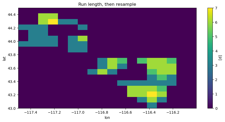
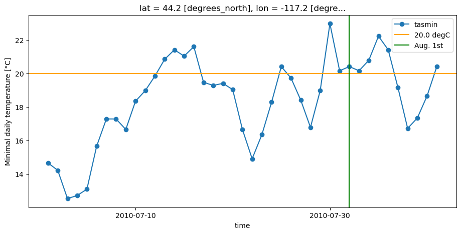
Let’s focus on the point \((-117.21075, 44.29087)\), which has a maximum wave length of four (4) or seven (7), depending on whether resampling occurs before or after the run length algorithm.

Plotting the values of tasmin in July and early August, we see a sequence of seven hot minimal temperatures at the end of July that surpass the threshold to qualify for a heat wave.

1. If resampling occurs first, and we first separate the periods in months, the run length algorithms will only look for sequences of hot days within the month of July and will exclude the last 3 days of this sequence of 7 days.

2. Using the run length algorithm before resampling looks for sequences of hot days in all the dataset given (temperatures from May 1, 2010 to Aug. 31, 2010) and then subdivides these sequences in the months where they have started. Since it starts in July, this sequence is registered as counts for a heat wave of seven days happening in July.

This also implies that the first 3 days of August which belong in this sequence of seven days will be counted as a sequence in August with the first method, but not with the second.

from xclim.core.units import convert_units_to

# Select a spatial point of interest in July-early August
lon_i, lat_i = -117.21075, 44.29087
tn_pt = tn.sel(time=slice("2010-07-01", "2010-08-05")).sel(lat=lat_i, lon=lon_i)
tn_pt = convert_units_to(tn_pt, "degC")

tn_pt.plot(marker="o", label="tasmin")
plt.axhline(y=convert_units_to(thresh_tn, "degC"), color="orange", label=thresh_tn)
plt.axvline(x=["2010-08-01"], color="green", label="Aug. 1st")
plt.legend()
plt.show()

Lazy computation - Nothing has been computed so far !

If you look at the output of those operations, they’re identified as dask.array objects. What happens is that dask creates a chain of operations that, when executed, will yield the values we want. We have thus far only created a schedule of tasks with a small preview and not done any actual computations. You can trigger computations by using the load or compute method, or writing the output to disk via to_netcdf. Of course, calling .plot() will also trigger the computation.

%%time
output_file = output_folder / "test_tx_max.nc"
dsOut.to_netcdf(output_file)

---------------------------------------------------------------------------
NameError                                 Traceback (most recent call last)
File <timed exec>:2

NameError: name 'dsOut' is not defined

(Times may of course vary depending on the machine and the Client settings)

Performance tips

Optimizing the chunk size

You can improve performance by being smart about chunk sizes. If chunks are too small, there is a lot of time lost in overhead. If chunks are too large, you may end up exceeding the individual worker memory limit.

print(ds2.chunks["time"])

(330, 365, 365, 365, 365, 365, 365, 365, 365, 365, 365, 37)

# rechunk data in memory for the entire grid
ds2c = ds2.chunk(chunks={"time": 4 * 365})
print(ds2c.chunks["time"])

(1460, 1460, 1097)

%%time
out = xclim.atmos.tx_max(ds2c.tasmax, freq="YS")
ds_out = xr.Dataset(data_vars=None, coords=out.coords, attrs=ds.attrs)
ds_out[out.name] = out

output_file = output_folder / "test_tx_max.nc"
ds_out.to_netcdf(output_file)

/home/docs/checkouts/readthedocs.org/user_builds/xclim/conda/stable/lib/python3.12/site-packages/xclim/core/cfchecks.py:42: UserWarning: Variable does not have a `cell_methods` attribute.
  _check_cell_methods(

CPU times: user 351 ms, sys: 39.3 ms, total: 391 ms
Wall time: 11.1 s

Loading the data in memory

If the dataset is relatively small, it might be more efficient to simply load the data into the memory and use numpy arrays instead of dask arrays.

ds4 = ds3.load()

Unit handling in xclim

A lot of effort has been placed into automatic handling of input data units. xclim will automatically detect the input variable(s) units (e.g. °C versus °K or mm/s versus mm/day etc.) and adjust on-the-fly in order to calculate indices in the consistent manner. This comes with the obvious caveat that input data requires metadata attribute for units.

The Units Handling page goes more into detail on how unit conversion can easily be done.

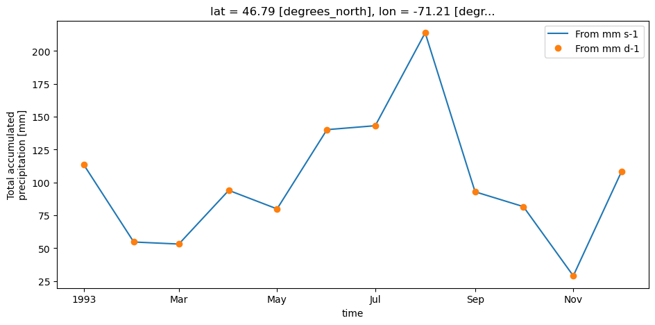
In the example below, we compute weekly total precipitation in mm using inputs of mm/s and mm/d. As we can see, the output is identical.

# Compute with the original mm s-1 data
out1 = xclim.atmos.precip_accumulation(ds4.pr, freq="MS")
# Create a copy of the data converted to mm d-1
pr_mmd = ds4.pr * 3600 * 24
pr_mmd.attrs["units"] = "mm d-1"
out2 = xclim.atmos.precip_accumulation(pr_mmd, freq="MS")

/home/docs/checkouts/readthedocs.org/user_builds/xclim/conda/stable/lib/python3.12/site-packages/xclim/core/cfchecks.py:42: UserWarning: Variable does not have a `cell_methods` attribute.
  _check_cell_methods(
/home/docs/checkouts/readthedocs.org/user_builds/xclim/conda/stable/lib/python3.12/site-packages/xclim/core/cfchecks.py:46: UserWarning: Variable has a non-conforming standard_name: Got `lwe_precipitation_rate`, expected `['precipitation_flux']`
  check_valid(vardata, "standard_name", data["standard_name"])
/home/docs/checkouts/readthedocs.org/user_builds/xclim/conda/stable/lib/python3.12/site-packages/xclim/core/cfchecks.py:42: UserWarning: Variable does not have a `cell_methods` attribute.
  _check_cell_methods(
/home/docs/checkouts/readthedocs.org/user_builds/xclim/conda/stable/lib/python3.12/site-packages/xclim/core/cfchecks.py:46: UserWarning: Variable does not have a `standard_name` attribute.
  check_valid(vardata, "standard_name", data["standard_name"])

plt.figure()
out1.plot(label="From mm s-1", linestyle="-")
out2.plot(label="From mm d-1", linestyle="none", marker="o")
plt.legend()
plt.show()

Threshold indices

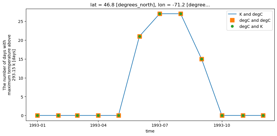
xclim unit handling also applies to threshold indicators. Users can provide threshold in units of choice and xclim will adjust automatically. For example, determining the number of days with tasmax > 20 °C, users can define a threshold input of "20 C" or "20 degC" even if input data is in Kelvin. Alternatively, users can even provide a threshold in Kelvin ("293.15 K", if they really wanted to).

# Create a copy of the data converted to C
tasmax_C = ds4.tasmax - 273.15
tasmax_C.attrs["units"] = "C"

# Using Kelvin data, threshold in Celsius
out1 = xclim.atmos.tx_days_above(ds4.tasmax, thresh="20 C", freq="MS")

# Using Celsius data
out2 = xclim.atmos.tx_days_above(tasmax_C, thresh="20 C", freq="MS")

# Using Celsius but with threshold in Kelvin
out3 = xclim.atmos.tx_days_above(tasmax_C, thresh="293.15 K", freq="MS")

# Plot and see that it's all identical:
plt.figure()
out1.plot(label="K and degC", linestyle="-")
out2.plot(label="degC and degC", marker="s", markersize=10, linestyle="none")
out3.plot(label="degC and K", marker="o", linestyle="none")
plt.legend()
plt.show()

/home/docs/checkouts/readthedocs.org/user_builds/xclim/conda/stable/lib/python3.12/site-packages/xclim/core/cfchecks.py:42: UserWarning: Variable does not have a `cell_methods` attribute.
  _check_cell_methods(
/home/docs/checkouts/readthedocs.org/user_builds/xclim/conda/stable/lib/python3.12/site-packages/xclim/core/cfchecks.py:42: UserWarning: Variable does not have a `cell_methods` attribute.
  _check_cell_methods(
/home/docs/checkouts/readthedocs.org/user_builds/xclim/conda/stable/lib/python3.12/site-packages/xclim/core/cfchecks.py:46: UserWarning: Variable does not have a `standard_name` attribute.
  check_valid(vardata, "standard_name", data["standard_name"])
/home/docs/checkouts/readthedocs.org/user_builds/xclim/conda/stable/lib/python3.12/site-packages/xclim/core/cfchecks.py:42: UserWarning: Variable does not have a `cell_methods` attribute.
  _check_cell_methods(
/home/docs/checkouts/readthedocs.org/user_builds/xclim/conda/stable/lib/python3.12/site-packages/xclim/core/cfchecks.py:46: UserWarning: Variable does not have a `standard_name` attribute.
  check_valid(vardata, "standard_name", data["standard_name"])

Spatially varying thresholds

Thresholds can also be passed as DataArrays instead of single scalar values, allowing the computation to depend on one or more non-temporal dimensions. The units attribute must be set.

Going back to the initial ds, we’ll subset it and compute the length of the heat wave according to thresholds that vary along the latitude and longitude.

ds5 = ds.sel(time=slice("1950", "1960"), lat=slice(50, 46), lon=slice(-75, -71))
ds5

<xarray.Dataset> Size: 111MB
Dimensions:  (lat: 48, lon: 48, time: 4018)
Coordinates:
  * lat      (lat) float32 192B 49.96 49.87 49.79 49.71 ... 46.21 46.12 46.04
  * lon      (lon) float32 192B -74.96 -74.88 -74.8 ... -71.21 -71.13 -71.05
  * time     (time) datetime64[ns] 32kB 1950-01-01 1950-01-02 ... 1960-12-31
Data variables:
    tasmin   (time, lat, lon) float32 37MB dask.array<chunksize=(365, 48, 48), meta=np.ndarray>
    tasmax   (time, lat, lon) float32 37MB dask.array<chunksize=(365, 48, 48), meta=np.ndarray>
    pr       (time, lat, lon) float32 37MB dask.array<chunksize=(365, 48, 48), meta=np.ndarray>
Attributes: (12/26)
    Conventions:                CF-1.5
    title:                      Ouranos standard ensemble of bias-adjusted cl...
    history:                    CMIP5 compliant file produced from raw ACCESS...
    institution:                Ouranos Consortium on Regional Climatology an...
    source:                     ACCESS1-3 2011. Atmosphere: AGCM v1.0 (N96 gr...
    driving_experiment:         historical,rcp85
    ...                         ...
    frequency:                  day
    modeling_realm:             atmos
    target_dataset:             CANADA : ANUSPLIN interpolated Canada daily 3...
    target_dataset_references:  CANADA : https://doi.org/10.1175/2011BAMS3132...
    driving_institution:        Commonwealth Scientific and Industrial Resear...
    driving_institute_id:       CSIRO-BOM

xarray.Dataset

• Dimensions:
  • lat: 48
  • lon: 48
  • time: 4018
• Coordinates: (3)
  • lat
    (lat)
    float32
    49.96 49.87 49.79 ... 46.12 46.04

    axis :

    Y

    units :

    degrees_north

    long_name :

    latitude

    standard_name :

    latitude

    array([49.95731, 49.87398, 49.79065, 49.70732, 49.62399, 49.54066, 49.45733,
           49.374  , 49.29067, 49.20734, 49.12401, 49.04068, 48.95735, 48.87402,
           48.79069, 48.70736, 48.62403, 48.5407 , 48.45737, 48.37404, 48.29071,
           48.20738, 48.12405, 48.04072, 47.95739, 47.87406, 47.79073, 47.7074 ,
           47.62407, 47.54074, 47.45741, 47.37408, 47.29075, 47.20742, 47.12409,
           47.04076, 46.95743, 46.8741 , 46.79077, 46.70744, 46.62411, 46.54078,
           46.45745, 46.37412, 46.29079, 46.20746, 46.12413, 46.0408 ],
          dtype=float32)

  • lon
    (lon)
    float32
    -74.96 -74.88 ... -71.13 -71.05

    axis :

    X

    units :

    degrees_east

    long_name :

    longitude

    standard_name :

    longitude

    array([-74.96244, -74.87911, -74.79578, -74.71245, -74.62912, -74.54579,
           -74.46246, -74.37913, -74.2958 , -74.21247, -74.12914, -74.04581,
           -73.96248, -73.87915, -73.79582, -73.71249, -73.62916, -73.54583,
           -73.4625 , -73.37917, -73.29584, -73.21251, -73.12918, -73.04585,
           -72.96252, -72.87919, -72.79586, -72.71253, -72.6292 , -72.54587,
           -72.46254, -72.37921, -72.29588, -72.21255, -72.12922, -72.04589,
           -71.96256, -71.87923, -71.7959 , -71.71257, -71.62924, -71.54591,
           -71.46258, -71.37925, -71.29592, -71.21259, -71.12926, -71.04593],
          dtype=float32)

  • time
    (time)
    datetime64[ns]
    1950-01-01 ... 1960-12-31

    axis :

    T

    long_name :

    time

    standard_name :

    time

    array(['1950-01-01T00:00:00.000000000', '1950-01-02T00:00:00.000000000',
           '1950-01-03T00:00:00.000000000', ..., '1960-12-29T00:00:00.000000000',
           '1960-12-30T00:00:00.000000000', '1960-12-31T00:00:00.000000000'],
          dtype='datetime64[ns]')

• Data variables: (3)
  • tasmin
    (time, lat, lon)
    float32
    dask.array<chunksize=(365, 48, 48), meta=np.ndarray>

    long_name :

    air_temperature

    standard_name :

    air_temperature

    units :

    K

    _ChunkSizes :

    [256 16 16]

    Array Chunk Bytes 35.31 MiB 3.21 MiB Shape (4018, 48, 48) (365, 48, 48) Dask graph 12 chunks in 3 graph layers Data type float32 numpy.ndarray

  • tasmax
    (time, lat, lon)
    float32
    dask.array<chunksize=(365, 48, 48), meta=np.ndarray>

    long_name :

    air_temperature

    standard_name :

    air_temperature

    units :

    K

    _ChunkSizes :

    [256 16 16]

    Array Chunk Bytes 35.31 MiB 3.21 MiB Shape (4018, 48, 48) (365, 48, 48) Dask graph 12 chunks in 3 graph layers Data type float32 numpy.ndarray

  • pr
    (time, lat, lon)
    float32
    dask.array<chunksize=(365, 48, 48), meta=np.ndarray>

    long_name :

    lwe_precipitation_rate

    standard_name :

    lwe_precipitation_rate

    units :

    mm s-1

    _ChunkSizes :

    [256 16 16]

    Array Chunk Bytes 35.31 MiB 3.21 MiB Shape (4018, 48, 48) (365, 48, 48) Dask graph 12 chunks in 3 graph layers Data type float32 numpy.ndarray

• Indexes: (3)
  • lat
    PandasIndex

    PandasIndex(Index([ 49.95730972290039,  49.87398147583008,   49.7906494140625,
            49.70732116699219,  49.62398910522461,   49.5406608581543,
            49.45732879638672, 49.374000549316406,  49.29066848754883,
           49.207340240478516,  49.12400817871094, 49.040679931640625,
            48.95735168457031, 48.874019622802734,  48.79069137573242,
           48.707359313964844,  48.62403106689453,  48.54069900512695,
            48.45737075805664,  48.37403869628906,  48.29071044921875,
            48.20737838745117,  48.12405014038086,  48.04072189331055,
            47.95738983154297, 47.874061584472656,  47.79072952270508,
           47.707401275634766,  47.62406921386719, 47.540740966796875,
             47.4574089050293, 47.374080657958984, 47.290748596191406,
           47.207420349121094, 47.124088287353516,   47.0407600402832,
            46.95743179321289,  46.87409973144531,    46.790771484375,
            46.70743942260742,  46.62411117553711,  46.54077911376953,
            46.45745086669922,  46.37411880493164,  46.29079055786133,
            46.20745849609375,  46.12413024902344,  46.04079818725586],
          dtype='float32', name='lat'))

  • lon
    PandasIndex

    PandasIndex(Index([-74.96244049072266, -74.87911224365234,  -74.7957763671875,
           -74.71244812011719, -74.62911987304688, -74.54579162597656,
           -74.46246337890625,  -74.3791275024414,  -74.2957992553711,
           -74.21247100830078, -74.12914276123047, -74.04580688476562,
           -73.96247863769531,   -73.879150390625, -73.79582214355469,
           -73.71248626708984, -73.62915802001953, -73.54582977294922,
            -73.4625015258789,  -73.3791732788086, -73.29583740234375,
           -73.21250915527344, -73.12918090820312, -73.04585266113281,
           -72.96251678466797, -72.87918853759766, -72.79586029052734,
           -72.71253204345703, -72.62920379638672, -72.54586791992188,
           -72.46253967285156, -72.37921142578125, -72.29588317871094,
            -72.2125473022461, -72.12921905517578, -72.04589080810547,
           -71.96256256103516, -71.87922668457031,     -71.7958984375,
           -71.71257019042969, -71.62924194335938, -71.54591369628906,
           -71.46257781982422,  -71.3792495727539,  -71.2959213256836,
           -71.21259307861328, -71.12925720214844, -71.04592895507812],
          dtype='float32', name='lon'))

  • time
    PandasIndex

    PandasIndex(DatetimeIndex(['1950-01-01', '1950-01-02', '1950-01-03', '1950-01-04',
                   '1950-01-05', '1950-01-06', '1950-01-07', '1950-01-08',
                   '1950-01-09', '1950-01-10',
                   ...
                   '1960-12-22', '1960-12-23', '1960-12-24', '1960-12-25',
                   '1960-12-26', '1960-12-27', '1960-12-28', '1960-12-29',
                   '1960-12-30', '1960-12-31'],
                  dtype='datetime64[ns]', name='time', length=4018, freq=None))

• Attributes: (26)

  Conventions :

  CF-1.5

  title :

  Ouranos standard ensemble of bias-adjusted climate scenarios version 1.0 (cb-oura-1.0)

  history :

  CMIP5 compliant file produced from raw ACCESS model output using the ACCESS Post-Processor and CMOR2. 2012-04-03T09:00:00Z CMOR rewrote data to comply with CF standards and CMIP5 requirements. Fri Apr 13 09:55:49 2012: forcing attribute modified to correct value Fri Apr 13 12:29:43 2012: corrected model_id from ACCESS1-3 to ACCESS1.3 Mon Jul 2 11:11:41 2012: updated version number to v20120413. 2016-01-18T16:42:49: Interpolate to nrcan_livneh grid. 2016-02-10T09:49:59: Bias correction using nrcan_livneh.

  institution :

  Ouranos Consortium on Regional Climatology and Adaptation to Climate Change

  source :

  ACCESS1-3 2011. Atmosphere: AGCM v1.0 (N96 grid-point, 1.875 degrees EW x approx 1.25 degree NS, 38 levels); ocean: NOAA/GFDL MOM4p1 (nominal 1.0 degree EW x 1.0 degrees NS, tripolar north of 65N, equatorial refinement to 1/3 degree from 10S to 10 N, cosine dependent NS south of 25S, 50 levels); sea ice: CICE4.1 (nominal 1.0 degree EW x 1.0 degrees NS, tripolar north of 65N, equatorial refinement to 1/3 degree from 10S to 10 N, cosine dependent NS south of 25S); land: CABLE1.0 (1.875 degree EW x 1.25 degree NS, 6 levels 30-day moving window 50-bins quantile mapping with detrending.

  driving_experiment :

  historical,rcp85

  institute_id :

  Ouranos

  dataset_id :

  cb-oura-1.0

  type :

  GCM

  processing :

  bias_adjusted

  dataset_description :

  https://www.ouranos.ca/publication-scientifique/FicheLoganGauvin2016_EN.pdf

  abstract :

  In order to satisfy growing demand and ensure the availability of climate scenarios that meet the needs of vulnerability, impact and adaptation (VIA) studies, a standard ensemble of bias-adjusted climate scenarios has been produced. Resulting climate scenarios are constructed using outputs of 11 individual global climate models and two future greenhouse gas emissions scenarios (RCP 4.5 and RCP 8.5) to cover the range of plausible of future changes and post-processed to refine the spatial scales and correct biases. The selection of a subset of simulations from the entire CMIP5 ensemble was carried out using a cluster analysis. The selection criteria include projected monthly changes in maximum and minimum temperatures as well as in total precipitations for two future horizons (2041 to 2070 and 2071 to 2100)

  driving_model_id :

  ACCESS1-3

  bias_adjustment_method :

  1D-Quantile Mapping

  bias_adjustment_reference :

  http://doi.org/10.1002/2015JD023890

  project_id :

  CMIP5

  license_type :

  permissive non-commercial

  license :

  Creative Commons Attribution-NonCommercial 4.0 International Public License: https://creativecommons.org/licenses/by-nc/4.0/legalcode

  terms_of_use :

  In addition to the provided licence, the data used for the realization of climate scenarios are subject to the conditions of use of each organization that is the source of this data, and that you must respect. For more details, please refer to:https://pcmdi.llnl.gov/mips/cmip5/terms-of-use.html

  attribution :

  Use of this dataset should be acknowledged as 'Data produced and provided by the Ouranos Consortium on Regional Climatology and Adaptation to Climate Change'. Furthermore, the modeling groups from which the bias-adjusted climate scenarios were consrtucted must also be acknowledged, please refer to: The Coupled Model Intercomparison Project https://pcmdi.llnl.gov/mips/cmip5/citation.html

  frequency :

  day

  modeling_realm :

  atmos

  target_dataset :

  CANADA : ANUSPLIN interpolated Canada daily 300 arc second climate grids; USA : Livneh_et_al_2013

  target_dataset_references :

  CANADA : https://doi.org/10.1175/2011BAMS3132.1; USA : https://doi.org/10.1175/JCLI-D-12-00508.1

  driving_institution :

  Commonwealth Scientific and Industrial Research Organization (CSIRO) and Bureau of Meteorology (BOM), Australia

  driving_institute_id :

  CSIRO-BOM

# The tasmin threshold is 7°C for the northern half of the domain and 11°C for the southern half.
# (notice that the lat coordinate is in decreasing order : from north to south)
thresh_tasmin = xr.DataArray(
    [7] * 24 + [11] * 24, dims=("lat",), coords={"lat": ds5.lat}, attrs={"units": "°C"}
)
# The tasmax threshold is 17°C for the western half of the domain and 21°C for the eastern half.
thresh_tasmax = xr.DataArray(
    [17] * 24 + [21] * 24, dims=("lon",), coords={"lon": ds5.lon}, attrs={"units": "°C"}
)

out_hw2d = xclim.atmos.heat_wave_total_length(
    tasmin=ds5.tasmin,
    tasmax=ds5.tasmax,
    thresh_tasmin=thresh_tasmin,
    thresh_tasmax=thresh_tasmax,
    freq="YS",
    window=3,
)

/home/docs/checkouts/readthedocs.org/user_builds/xclim/conda/stable/lib/python3.12/site-packages/xclim/core/cfchecks.py:42: UserWarning: Variable does not have a `cell_methods` attribute.
  _check_cell_methods(

The final map for year 1958, shows clear jumps across the 4 quadrants, which was expected with our space-dependent thresholds. Notice also how the long_name (printed on the colorbar label) mentions that the threshold comes from “an array”. This imprecise metadata is a consequence of using DataArray-derived thresholds.

out_hw2d.sel(time="1958").plot()
plt.show()