Unit Handling¶

[1]:

from __future__ import annotations

import matplotlib.pyplot as plt
import nc_time_axis  # noqa
import xarray as xr

import xclim
from xclim.core import units
from xclim.testing import open_dataset

# Set display to HTML style (optional)
xr.set_options(display_style="html", display_width=50)

%matplotlib inline
plt.rcParams["figure.figsize"] = (11, 5)

A lot of effort has been placed into automatic handling of input data units. xclim will automatically detect the input variable(s) units (e.g. °C versus K or mm/s versus mm/day etc.) and adjust on-the-fly in order to calculate indices in the consistent manner. This comes with the obvious caveat that input data requires a metadata attribute for units : the units attribute is required, and the standard_name can be useful for automatic conversions.

The main unit handling method is `xclim.core.units.convert_units_to <../xclim.core.rst#xclim.core.units.convert_units_to>`__ which can also be useful on its own. xclim relies on pint for unit handling and extends the units registry and formatting functions of cf-xarray.

Simple example: Temperature¶

[2]:

# See the Usage page for details on opening datasets, subsetting and resampling.
ds = xr.tutorial.load_dataset("air_temperature")
tas = ds.air.sel(lat=40, lon=270, method="nearest").resample(time="D").mean(keep_attrs=True)
print(tas.attrs["units"])

degK

Here, we convert our kelvin data to the very useful Fahrenheits:

[3]:

tas_F = units.convert_units_to(tas, "degF")
print(tas_F.attrs["units"])

°F

Threshold indices¶

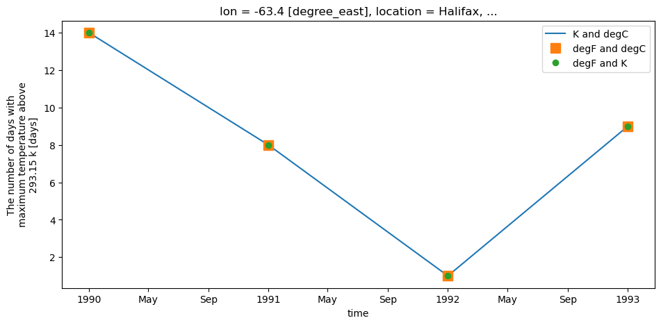
xclim unit handling also applies to threshold indicators. Users can provide threshold in units of choice and xclim will adjust automatically. For example, in order to determine the number of days with tasmax > 20 °C, users can define a threshold input of "20 C" or "20 degC" even if input data is in Kelvin. Alternatively, users can even provide a threshold in Kelvin ("293.15 K"), if they really wanted to.

[8]:

tasmaxK = ds.tasmax.sel(location="Halifax")
tasmaxF = units.convert_units_to(ds.tasmax.sel(location="Halifax"), "degF")

with xclim.set_options(cf_compliance="log"):
    # Using Kelvin data, threshold in Celsius
    out1 = xclim.atmos.tx_days_above(tasmax=tasmaxK, thresh="20 C", freq="YS")

    # Using Fahrenheit data, threshold in Celsius
    out2 = xclim.atmos.tx_days_above(tasmax=tasmaxF, thresh="20 C", freq="YS")

    # Using Fahrenheit data, with threshold in Kelvin
    out3 = xclim.atmos.tx_days_above(tasmax=tasmaxF, thresh="293.15 K", freq="YS")

# Plot and see that it's all identical:
plt.figure()
out1.plot(label="K and degC", linestyle="-")
out2.plot(label="degF and degC", marker="s", markersize=10, linestyle="none")
out3.plot(label="degF and K", marker="o", linestyle="none")
plt.legend()

[8]:

<matplotlib.legend.Legend at 0x7606c84810d0>

Sum and count indices¶

Many indices in xclim will either sum values or count events along the time dimension and over a period. As of version 0.24, unit handling dynamically infers what the sampling frequency and its corresponding unit is.

Indicators, on the other hand, do not have this flexibility and often expect input at a given frequency, more often daily than otherwise.

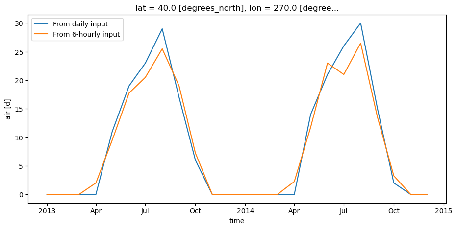
For example, we can run the tx_days_above on the 6-hourly test data, and it should return similar results as on the daily data, but in units of h (the base unit of the sampling frequency).

[9]:

ds = xr.tutorial.load_dataset("air_temperature")
tas_6h = ds.air.sel(lat=40, lon=270, method="nearest")  # no resampling, original data is 6-hourly
tas_D = tas_6h.resample(time="D").mean()
out1_h = xclim.indices.tx_days_above(tasmax=tas_6h, thresh="20 C", freq="MS")
out2_D = xclim.indices.tx_days_above(tasmax=tas_D, thresh="20 C", freq="MS")
out1_h

[9]:

<xarray.DataArray 'air' (time: 24)> Size: 192B
array([  0,   0,   0,  48, 228, 426, 492, 612, 456, 174,   0,   0,   0,
         0,   0,  54, 282, 552, 504, 636, 324,  78,   0,   0])
Coordinates:
  * time     (time) datetime64[ns] 192B 2013-01...
    lat      float32 4B 40.0
    lon      float32 4B 270.0
Attributes:
    long_name:     4xDaily Air temperature at s...
    units:         h
    precision:     2
    GRIB_id:       11
    GRIB_name:     TMP
    var_desc:      Air temperature
    dataset:       NMC Reanalysis
    level_desc:    Surface
    statistic:     Individual Obs
    parent_stat:   Other
    actual_range:  [185.16 322.1 ]

[10]:

out1_D = units.convert_units_to(out1_h, "d")
plt.figure()
out2_D.plot(label="From daily input", linestyle="-")
out1_D.plot(label="From 6-hourly input", linestyle="-")
plt.legend()

[10]:

<matplotlib.legend.Legend at 0x7606c844d400>

Temperature differences vs absolute temperature¶

Temperature anomalies and biases as well as degree-days indicators are all differences between temperatures. If we assign those differences units of degrees Celsius, then converting to Kelvins or Fahrenheits will yield nonsensical values. pint solves this using delta units such as delta_degC and delta_degF.

[11]:

# If we have a DataArray storing a temperature anomaly of 2°C,
# converting to Kelvin will yield a nonsensical value 0f 275.15.
# Fortunately, pint has delta units to represent temperature differences.
display(units.convert_units_to(xr.DataArray([2], attrs={"units": "delta_degC"}), "K"))

<xarray.DataArray (dim_0: 1)> Size: 8B
array([2])
Dimensions without coordinates: dim_0
Attributes:
    units:           K
    units_metadata:  temperature: unknown

The issue for xclim is that there are no equivalent delta units in the CF convention. To resolve this ambiguity, the CF convention recommends including a units_metadata attribute set to "temperature: difference", and this is supported in xclim as of version 0.52. The function units2pint interprets the units_metadata attribute and returns a pint delta unit as needed. To convert a pint delta unit to CF attributes, use the function pint2cfattrs, which returns a dictionary with the units and units_metadata attributes (pint2cfunits cannot support the convention because it only returns the unit string).

[12]:

delta = xr.DataArray([2], attrs={"units": "K", "units_metadata": "temperature: difference"})
units.convert_units_to(delta, "delta_degC")

[12]:

<xarray.DataArray (dim_0: 1)> Size: 8B
array([2.])
Dimensions without coordinates: dim_0
Attributes:
    units:           degC
    units_metadata:  temperature: difference

Other utilities¶

Many helper functions are defined in xclim.core.units, see Unit handling module.