Download this notebook from github.
Ensembles
An important aspect of climate models is that they are run multiple times with some initial perturbations to see how they replicate the natural variability of the climate. Through xclim.ensembles, xclim provides an easy interface to compute ensemble statistics on different members. Most methods perform checks and conversion on top of simpler xarray methods, providing an easier interface to use.
create_ensemble
Our first step is to create an ensemble. This method takes a list of files defining the same variables over the same coordinates and concatenates them into one dataset with an added dimension realization.
Using xarray a very simple way of creating an ensemble dataset would be :
import xarray

xarray.open_mfdataset(files, concat_dim='realization')
However, this is only successful when the dimensions of all the files are identical AND only if the calendar type of each netcdf file is the same
xclim’s create_ensemble() method overcomes these constraints, selecting the common time period to all files and assigns a standard calendar type to the dataset.
Input netcdf files still require equal spatial dimension size (e.g. lon, lat dimensions).
Given files all named ens_tas_m[member number].nc, we use glob to get a list of all those files.
[2]:
import glob

import xarray as xr

import xclim as xc

# Set display to HTML sytle (for fancy output)
xr.set_options(display_style="html", display_width=50)

import matplotlib.pyplot as plt

%matplotlib inline

from xclim import ensembles

ens = ensembles.create_ensemble(glob.glob("ens_tas_m*.nc")).load()
ens.close()
/home/docs/checkouts/readthedocs.org/user_builds/xclim/conda/v0.43.0/lib/python3.10/site-packages/xclim/indices/fire/_cffwis.py:207: NumbaDeprecationWarning: The 'nopython' keyword argument was not supplied to the 'numba.jit' decorator. The implicit default value for this argument is currently False, but it will be changed to True in Numba 0.59.0. See https://numba.readthedocs.io/en/stable/reference/deprecation.html#deprecation-of-object-mode-fall-back-behaviour-when-using-jit for details.
  def _day_length(lat: int | float, mth: int):  # pragma: no cover
/home/docs/checkouts/readthedocs.org/user_builds/xclim/conda/v0.43.0/lib/python3.10/site-packages/xclim/indices/fire/_cffwis.py:227: NumbaDeprecationWarning: The 'nopython' keyword argument was not supplied to the 'numba.jit' decorator. The implicit default value for this argument is currently False, but it will be changed to True in Numba 0.59.0. See https://numba.readthedocs.io/en/stable/reference/deprecation.html#deprecation-of-object-mode-fall-back-behaviour-when-using-jit for details.
  def _day_length_factor(lat: float, mth: int):  # pragma: no cover
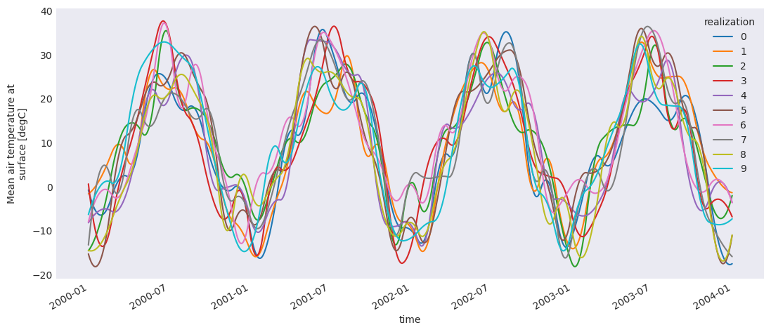
[3]:
plt.style.use("seaborn-v0_8-dark")
plt.rcParams["figure.figsize"] = (13, 5)
ens.tas.plot(hue="realization")
plt.show()
[4]:
ens.tas # Attributes of the first dataset to be opened are copied to the final output
[4]:
<xarray.DataArray 'tas' (realization: 10,
                         time: 1461)>
array([[ -0.74661228,  -1.14834882,  -1.53530599, ..., -17.61971376,
        -17.56192347, -17.48840648],
       [ -1.60477585,  -1.53196209,  -1.45478034, ...,  -1.29130334,
         -1.32623196,  -1.35751854],
       [-14.54425643, -14.41094884, -14.26933018, ...,  -2.77476123,
         -2.3891895 ,  -1.98746361],
       ...,
       [-13.22850295, -12.24738429, -11.29336498, ..., -15.67208672,
        -15.77506349, -15.87533369],
       [-14.46163135, -14.49828035, -14.52805846, ..., -12.03841506,
        -11.51116215, -10.95658622],
       [ -6.31010317,  -5.97253002,  -5.64234933, ...,  -7.47462733,
         -7.38653016,  -7.29506706]])
Coordinates:
  * time         (time) datetime64[ns] 2000-01-...
  * realization  (realization) int64 0 1 2 ... 8 9
Attributes:
    units:          degC
    standard_name:  air_temperature
    long_name:      Mean air temperature at sur...
title: tas of member 01Ensemble statistics
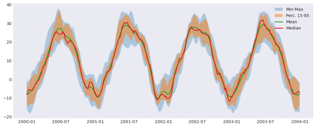
Beyond creating an ensemble dataset, the xclim.ensembles module contains functions for calculating statistics between realizations
Ensemble mean, standard-deviation, max & min
In the example below, we use xclim’s ensemble_mean_std_max_min() to calculate statistics across the 10 realizations in our test dataset. Output variables are created combining the original variable name tas with additional ending indicating the statistic calculated on the realization dimension : _mean, _stdev, _min, _max
The resulting output now contains 4 derived variables from the original single variable in our ensemble dataset.
[5]:
ens_stats = ensembles.ensemble_mean_std_max_min(ens)
ens_stats
[5]:
<xarray.Dataset>
Dimensions:    (time: 1461)
Coordinates:
  * time       (time) datetime64[ns] 2000-01-01...
Data variables:
    tas_mean   (time) float64 -8.165 ... -8.005
    tas_stdev  (time) float64 5.79 5.589 ... 5.398
    tas_max    (time) float64 0.633 ... -1.358
    tas_min    (time) float64 -15.26 ... -17.49
Attributes:
history: [2023-05-09 21:46:39] : Computati...Ensemble percentiles
Here, we use xclim’s ensemble_percentiles() to calculate percentile values across the 10 realizations. The output has now a percentiles dimension instead of realization. Split variables can be created instead, by specifying split=True (the variable name tas will be appended with _p{x}). Compared to NumPy’s percentile() and xarray’s quantile(), this method handles more efficiently dataset with invalid values and the chunking along the realization dimension (which
is automatic when dask arrays are used).
[6]:
ens_perc = ensembles.ensemble_percentiles(ens, values=[15, 50, 85], split=False)
ens_perc
[6]:
<xarray.Dataset>
Dimensions:      (time: 1461, percentiles: 3)
Coordinates:
  * time         (time) datetime64[ns] 2000-01-...
  * percentiles  (percentiles) int64 15 50 85
Data variables:
    tas          (time, percentiles) float64 -1...
Attributes:
    units:          degC
    standard_name:  air_temperature
    long_name:      Mean air temperature at sur...
    title:          tas of member 01
history: [2023-05-09 21:46:39] : Com...[7]:
fig, ax = plt.subplots()
ax.fill_between(
    ens_stats.time.values,
    ens_stats.tas_min,
    ens_stats.tas_max,
    alpha=0.3,
    label="Min-Max",
)
ax.fill_between(
    ens_perc.time.values,
    ens_perc.tas.sel(percentiles=15),
    ens_perc.tas.sel(percentiles=85),
    alpha=0.5,
    label="Perc. 15-85",
)
ax._get_lines.get_next_color()  # Hack to get different line
ax._get_lines.get_next_color()
ax.plot(ens_stats.time.values, ens_stats.tas_mean, linewidth=2, label="Mean")
ax.plot(
    ens_perc.time.values, ens_perc.tas.sel(percentiles=50), linewidth=2, label="Median"
)
ax.legend()
plt.show()