Download this notebook from github.
Workflow Examples
xclim is built on very powerful multiprocessing and distributed computation libraries, notably xarray and dask.
xarray is a python package making it easy to work with n-dimensional arrays. It labels axes with their names [time, lat, lon, level] instead of indices [0,1,2,3], reducing the likelihood of bugs and making the code easier to understand. One of the key strengths of xarray is that it knows how to deal with non-standard calendars (we’re looking at you, “360_days”) and can easily resample daily time series to weekly, monthly, seasonal or annual periods. Finally, xarray is
tightly inegrated with dask, a package that can automatically parallelize operations.
The following are a few examples to consult when using xclim to subset netCDF arrays and compute climate indicators, taking advantage of the parallel processing capabilities offered by xarray and dask. For more information about these projects, please see their documentation pages:
Environment configuration
[ ]:
# Imports for xclim and xarray
import numpy as np
import xarray as xr

import xclim as xc

xr.set_options(display_style="html")

import tempfile

# File handling libraries
import time
from pathlib import Path

# Output folder
output_folder = Path(tempfile.mkdtemp())
Setting up the Dask client: parallel processing
In this example, we are using the dask.distributed submodule. This is not installed by default in a basic xclim installation. Be sure to add distributed to your Python installation before setting up parallel processing operations!
First we create a pool of workers that will wait for jobs. The xarray library will automatically connect to these workers and and dispatch them jobs that can be run in parallel.
The dashboard link lets you see in real time how busy those workers are.
This step is not mandatory as dask will fall back to its “single machine scheduler” if a Client is not created. However, this default scheduler doesn’t allow you to set the number of threads or a memory limit and doesn’t start the dashboard, which can be quite useful to understand your task’s progress.
[ ]:
from distributed import Client

# Depending on your workstation specifications, you may need to adjust these values.
# On a single machine, n_workers=1 is usually better.
client = Client(n_workers=1, threads_per_worker=4, memory_limit="4GB")
client
Client
|
Cluster
|
Creating xarray datasets
To open a netCDF file with xarray, we use xr.open_dataset(<path to file>). By default, the entire file is stored in one chunk, so there is no parallelism. To trigger parallel computations, we need to explicitly specify the chunk size.
In this example, instead of opening a local file, we pass an OPeNDAP url to xarray. It retrieves the data automatically. Notice also that opening the dataset is quite fast. In fact, the data itself has not been downloaded yet, only the coordinates and the metadata. The downloads will be triggered only when the values need to be accessed directly.
dask’s parallelism is based on memory chunks. We need to tell xarray to split our netCDF array into chunks of a given size, and operations on each chunk of the array will automatically be dispatched to the workers.
[ ]:
data_url = "https://pavics.ouranos.ca/twitcher/ows/proxy/thredds/dodsC/datasets/simulations/bias_adjusted/cmip5/ouranos/cb-oura-1.0/day_ACCESS1-3_historical+rcp85_r1i1p1_na10kgrid_qm-moving-50bins-detrend_1950-2100.ncml"
[ ]:
# Chunking in memory along the time dimension.
# Note that the data type is a 'dask.array'. xarray will automatically use client workers.
ds = xr.open_dataset(
    data_url,
    chunks={"time": 365, "lat": 168, "lon": 150},
    drop_variables=["ts", "time_vectors"],
)
print(ds)
<xarray.Dataset>
Dimensions:  (lat: 320, lon: 797, time: 55152)
Coordinates:
  * lat      (lat) float32 66.62331 66.53998 66.45665 ... 40.12437 40.04104
  * lon      (lon) float32 -120.79394 -120.71061 ... -54.54659 -54.46326
  * time     (time) datetime64[ns] 1950-01-01 1950-01-02 ... 2100-12-31
Data variables:
    tasmin   (time, lat, lon) float32 dask.array<chunksize=(365, 168, 150), meta=np.ndarray>
    tasmax   (time, lat, lon) float32 dask.array<chunksize=(365, 168, 150), meta=np.ndarray>
    pr       (time, lat, lon) float32 dask.array<chunksize=(365, 168, 150), meta=np.ndarray>
Attributes:
    Conventions:                CF-1.5
    title:                      Ouranos standard ensemble of bias-adjusted cl...
    history:                    CMIP5 compliant file produced from raw ACCESS...
    institution:                Ouranos Consortium on Regional Climatology an...
    source:                     ACCESS1-3 2011. Atmosphere: AGCM v1.0 (N96 gr...
    driving_model:              ACCESS1-3
    driving_experiment:         historical,rcp85
    institute_id:               Ouranos
    type:                       GCM
    processing:                 bias_adjusted
    dataset_description:        https://www.ouranos.ca/publication-scientifiq...
    bias_adjustment_method:     1D-Quantile Mapping
    bias_adjustment_reference:  http://doi.org/10.1002/2015JD023890
    project_id:                 CMIP5
    licence_type:               permissive
    terms_of_use:               Terms of use at https://www.ouranos.ca/climat...
    attribution:                Use of this dataset should be acknowledged as...
    frequency:                  day
    modeling_realm:             atmos
    target_dataset:             CANADA : ANUSPLIN interpolated Canada daily 3...
    target_dataset_references:  CANADA : https://doi.org/10.1175/2011BAMS3132...
    driving_institution:        Commonwealth Scientific and Industrial Resear...
    driving_institute_id:       CSIRO-BOM
[ ]:
print(ds.tasmin.chunks)
((365, 365, 365, 365, 365, 365, 365, 365, 365, 365, 365, 365, 365, 365, 365, 365, 365, 365, 365, 365, 365, 365, 365, 365, 365, 365, 365, 365, 365, 365, 365, 365, 365, 365, 365, 365, 365, 365, 365, 365, 365, 365, 365, 365, 365, 365, 365, 365, 365, 365, 365, 365, 365, 365, 365, 365, 365, 365, 365, 365, 365, 365, 365, 365, 365, 365, 365, 365, 365, 365, 365, 365, 365, 365, 365, 365, 365, 365, 365, 365, 365, 365, 365, 365, 365, 365, 365, 365, 365, 365, 365, 365, 365, 365, 365, 365, 365, 365, 365, 365, 365, 365, 365, 365, 365, 365, 365, 365, 365, 365, 365, 365, 365, 365, 365, 365, 365, 365, 365, 365, 365, 365, 365, 365, 365, 365, 365, 365, 365, 365, 365, 365, 365, 365, 365, 365, 365, 365, 365, 365, 365, 365, 365, 365, 365, 365, 365, 365, 365, 365, 365, 37), (168, 152), (150, 150, 150, 150, 150, 47))
Multi-file datasets
NetCDF files are often split into periods to keep file size manageable. A single dataset can be split in dozens of individual files. xarray has a function open_mfdataset that can open and aggregate a list of files and construct a unique logical dataset. open_mfdataset can aggregate files over coordinates (time, lat, lon) and variables.
Note that opening a multi-file dataset automatically chunks the array (one chunk per file).
Note also that because
xarrayreads every file metadata to place it in a logical order, it can take a while to load.
[ ]:
## Create multi-file data & chunks
# ds = xr.open_mfdataset('/path/to/files*.nc')
Subsetting and selecting data with xarray
Usually, xclim users are encouraged to use the subsetting utilities of the clisops package. Here, we will reduce the size of our data using the methods implemented in xarray (docs here).
[ ]:
ds2 = ds.sel(lat=slice(50, 45), lon=slice(-70, -65), time=slice("2090", "2100"))
print(ds2.tasmin)
<xarray.DataArray 'tasmin' (time: 4017, lat: 60, lon: 60)>
dask.array<getitem, shape=(4017, 60, 60), dtype=float32, chunksize=(365, 60, 60), chunktype=numpy.ndarray>
Coordinates:
  * lat      (lat) float32 49.95731 49.87398 49.79065 ... 45.12417 45.04084
  * lon      (lon) float32 -69.96264 -69.87931 -69.79598 ... -65.1295 -65.04617
  * time     (time) datetime64[ns] 2090-01-01 2090-01-02 ... 2100-12-31
Attributes:
    long_name:      air_temperature
    standard_name:  air_temperature
    units:          K
    _ChunkSizes:    [256  16  16]
[ ]:
ds3 = ds.sel(lat=46.8, lon=-71.22, method="nearest").sel(time="1993")
print(ds3.tasmin)
Climate index calculation & resampling frequencies
xclim has two layers for the calculation of indicators. The bottom layer is composed of a list of functions that take one or more xarray.DataArray’s as input and return an xarray.DataArray as output. You’ll find these functions in xclim.indices. The indicator’s logic is contained in this function, as well as some unit handling, but it doesn’t perform any data consistency checks (like if the time frequency is daily), and doesn’t not adjust the metadata of the output array.
The second layer are class instances that you’ll find organized by realm. So far, there are three realms available in xclim.atmos, xclim.seaIce and xclim.land, the first one being the most exhaustive. Before running computations, these classes check if the input data is a daily average of the expected variable:
If an indicator expects a daily mean and you pass it a daily max, a
warningwill be raised.After the computation, it also checks the number of values per period to make sure there are not missing values or
NaNin the input data. If there are, the output is going to be set toNaN. Ex. : If the indicator performs a yearly resampling but there are only 350 non-NaNvalues in one given year in the input data, that year’s output will beNaN.The output units are set correctly as well as other properties of the output array, complying as much as possible with CF conventions.
For new users, we suggest you use the classes found in xclim.atmos and others. If you know what you’re doing and you want to circumvent the built-in checks, then you can use the xclim.indices directly.
Almost all xclim indicators convert daily data to lower time frequencies, such as seasonal or annual values. This is done using xarray.DataArray.resample method. Resampling creates a grouped object over which you apply a reduction operation (e.g. mean, min, max). The list of available frequency is given in the link below, but the most often used are:
YS: annual starting in JanuaryYS-JUL: annual starting in JulyMS: monthlyQS-DEC: seasonal starting in December
More info about this specification can be found in pandas’ documentation
Note - not all offsets in the link are supported by cftime objects in xarray.
In the example below, we’re computing the annual maximum temperature of the daily maximum temperature (tx_max).
[ ]:
out = xc.atmos.tx_max(ds2.tasmax, freq="YS")
print(out)
/home/phobos/Python/xclim/xclim/indicators/atmos/_temperature.py:87: UserWarning: Variable does not have a `cell_methods` attribute.
  cfchecks.check_valid(tasmax, "cell_methods", "*time: maximum within days*")
<xarray.DataArray 'tx_max' (time: 11, lat: 60, lon: 60)>
dask.array<where, shape=(11, 60, 60), dtype=float32, chunksize=(1, 60, 60), chunktype=numpy.ndarray>
Coordinates:
  * time     (time) datetime64[ns] 2090-01-01 2091-01-01 ... 2100-01-01
  * lat      (lat) float32 49.95731 49.87398 49.79065 ... 45.12417 45.04084
  * lon      (lon) float32 -69.96264 -69.87931 -69.79598 ... -65.1295 -65.04617
Attributes:
    long_name:      Maximum daily maximum temperature
    standard_name:  air_temperature
    units:          K
    _ChunkSizes:    [256  16  16]
    cell_methods:    time: maximum within days time: maximum over days
    xclim_history:  [2021-02-15 17:08:48] tx_max: tx_max(tasmax=<array>, freq...
    description:    Annual maximum of daily maximum temperature.
If you execute the cell above, you’ll see that this operation is quite fast. This a feature coming from dask. Read Lazy computation further down.
Comparison of atmos vs indices modules
Using the xclim.indices module performs not checks and only fills the units attribute.
[ ]:
out = xc.indices.tx_days_above(ds2.tasmax, thresh="30 C", freq="YS")
print(out)
<xarray.DataArray 'tasmax' (time: 11, lat: 60, lon: 60)>
dask.array<mul, shape=(11, 60, 60), dtype=int64, chunksize=(1, 60, 60), chunktype=numpy.ndarray>
Coordinates:
  * time     (time) datetime64[ns] 2090-01-01 2091-01-01 ... 2100-01-01
  * lat      (lat) float32 49.95731 49.87398 49.79065 ... 45.12417 45.04084
  * lon      (lon) float32 -69.96264 -69.87931 -69.79598 ... -65.1295 -65.04617
Attributes:
    units:    d
With xclim.atmos, checks are performed and many CF-compliant attributes are added:
[ ]:
out = xc.atmos.tx_days_above(ds2.tasmax, thresh="30 C", freq="YS")
print(out)
<xarray.DataArray 'tx_days_above' (time: 11, lat: 60, lon: 60)>
dask.array<where, shape=(11, 60, 60), dtype=float64, chunksize=(1, 60, 60), chunktype=numpy.ndarray>
Coordinates:
  * time     (time) datetime64[ns] 2090-01-01 2091-01-01 ... 2100-01-01
  * lat      (lat) float32 49.95731 49.87398 49.79065 ... 45.12417 45.04084
  * lon      (lon) float32 -69.96264 -69.87931 -69.79598 ... -65.1295 -65.04617
Attributes:
    units:          days
    cell_methods:    time: maximum within days time: sum over days
    xclim_history:  [2021-02-15 17:08:49] tx_days_above: tx_days_above(tasmax...
    standard_name:  number_of_days_with_air_temperature_above_threshold
    long_name:      Number of days with tmax > 30 c
    description:    Annual number of days where daily maximum temperature exc...
/home/phobos/Python/xclim/xclim/indicators/atmos/_temperature.py:87: UserWarning: Variable does not have a `cell_methods` attribute.
  cfchecks.check_valid(tasmax, "cell_methods", "*time: maximum within days*")
[ ]:
# We have created an xarray data-array - We can insert this into an output xr.Dataset object with a copy of the original dataset global attrs
dsOut = xr.Dataset(attrs=ds2.attrs)

# Add our climate index as a data variable to the dataset
dsOut[out.name] = out
print(dsOut)
<xarray.Dataset>
Dimensions:        (lat: 60, lon: 60, time: 11)
Coordinates:
  * time           (time) datetime64[ns] 2090-01-01 2091-01-01 ... 2100-01-01
  * lat            (lat) float32 49.95731 49.87398 ... 45.12417 45.04084
  * lon            (lon) float32 -69.96264 -69.87931 ... -65.1295 -65.04617
Data variables:
    tx_days_above  (time, lat, lon) float64 dask.array<chunksize=(1, 60, 60), meta=np.ndarray>
Attributes:
    Conventions:                CF-1.5
    title:                      Ouranos standard ensemble of bias-adjusted cl...
    history:                    CMIP5 compliant file produced from raw ACCESS...
    institution:                Ouranos Consortium on Regional Climatology an...
    source:                     ACCESS1-3 2011. Atmosphere: AGCM v1.0 (N96 gr...
    driving_model:              ACCESS1-3
    driving_experiment:         historical,rcp85
    institute_id:               Ouranos
    type:                       GCM
    processing:                 bias_adjusted
    dataset_description:        https://www.ouranos.ca/publication-scientifiq...
    bias_adjustment_method:     1D-Quantile Mapping
    bias_adjustment_reference:  http://doi.org/10.1002/2015JD023890
    project_id:                 CMIP5
    licence_type:               permissive
    terms_of_use:               Terms of use at https://www.ouranos.ca/climat...
    attribution:                Use of this dataset should be acknowledged as...
    frequency:                  day
    modeling_realm:             atmos
    target_dataset:             CANADA : ANUSPLIN interpolated Canada daily 3...
    target_dataset_references:  CANADA : https://doi.org/10.1175/2011BAMS3132...
    driving_institution:        Commonwealth Scientific and Industrial Resear...
    driving_institute_id:       CSIRO-BOM
Lazy computation - Nothing has been computed so far !
If you look at the output of those operations, they’re identified as dask.array objects. What happens is that dask creates a chain of operations that when executed, will yield the values we want. We have thus far only created a schedule of tasks with a small preview and not done any actual computations. You can trigger computations by using the load or compute method, or writing the output to disk via to_netcdf. Of course, calling .plot() will also trigger the
computation.
[ ]:
%%time
output_file = output_folder / "test_tx_max.nc"
dsOut.to_netcdf(output_file)
CPU times: user 1.1 s, sys: 74.4 ms, total: 1.17 s
Wall time: 14.4 s
(Times may of course vary depending on the machine and the Client settings)
Performance tips
Optimizing the chunk size
You can improve performance by being smart about chunk sizes. If chunks are too small, there is a lot of time lost in overhead. If chunks are too large, you may end up exceeding the individual worker memory limit.
[ ]:
print(ds2.chunks["time"])
(330, 365, 365, 365, 365, 365, 365, 365, 365, 365, 365, 37)
[ ]:
# rechunk data in memory for the entire grid
ds2c = ds2.chunk(chunks={"time": 4 * 365})
print(ds2c.chunks["time"])
(1460, 1460, 1097)
[ ]:
%%time
out = xc.atmos.tx_max(ds2c.tasmax, freq="YS")
dsOut = xr.Dataset(data_vars=None, coords=out.coords, attrs=ds.attrs)
dsOut[out.name] = out

output_file = output_folder / "test_tx_max.nc"
dsOut.to_netcdf(output_file)
/home/phobos/Python/xclim/xclim/indicators/atmos/_temperature.py:87: UserWarning: Variable does not have a `cell_methods` attribute.
  cfchecks.check_valid(tasmax, "cell_methods", "*time: maximum within days*")
CPU times: user 582 ms, sys: 75.1 ms, total: 657 ms
Wall time: 5.42 s
Loading the data in memory
If the dataset is relatively small, it might be more efficient to simply load the data into the memory and use numpy arrays instead of dask arrays.
[ ]:
ds4 = ds3.load()
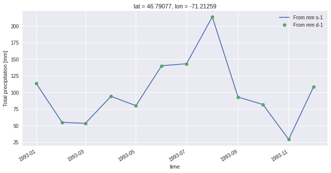
Unit handling in xclim
A lot of effort has been placed into automatic handling of input data units. xclim will automatically detect the input variable(s) units (e.g. °C versus °K or mm/s versus mm/day etc.) and adjust on-the-fly in order to calculate indices in the consistent manner. This comes with the obvious caveat that input data requires metadata attribute for units.
In the example below, we compute weekly total precipitation in mm using inputs of mm/s and mm/d. As you see, the output is identical.
[ ]:
# Compute with the original mm s-1 data
out1 = xc.atmos.precip_accumulation(ds4.pr, freq="MS")
# Create a copy of the data converted to mm d-1
pr_mmd = ds4.pr * 3600 * 24
pr_mmd.attrs["units"] = "mm d-1"
out2 = xc.atmos.precip_accumulation(pr_mmd, freq="MS")
[ ]:
# import plotting stuff
import matplotlib.pyplot as plt

%matplotlib inline
plt.style.use("seaborn")
plt.rcParams["figure.figsize"] = (11, 5)
[ ]:
plt.figure()
out1.plot(label="From mm s-1", linestyle="-")
out2.plot(label="From mm d-1", linestyle="none", marker="o")
plt.legend()
<matplotlib.legend.Legend at 0x7fb6e8360b50>
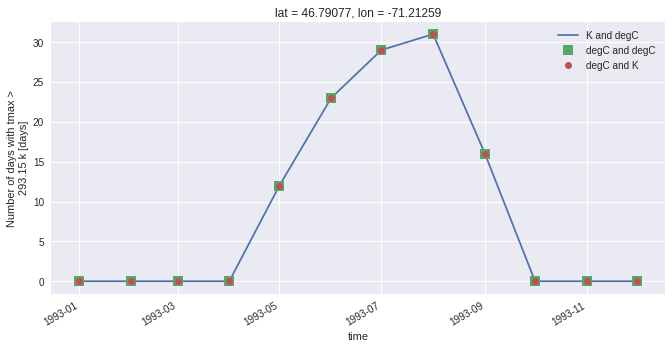
Threshold indices
xclim unit handling also applies to threshold indicators. Users can provide threshold in units of choice and xclim will adjust automatically. For example determining the number of days with tasmax > 20°C users can define a threshold input of ‘20 C’ or ‘20 degC’ even if input data is in Kelvin. Alernatively users can even provide a threshold in Kelvin ‘293.15 K’ (if they really wanted to).
[ ]:
# Create a copy of the data converted to C
tasmax_C = ds4.tasmax - 273.15
tasmax_C.attrs["units"] = "C"

# Using Kelvin data, threshold in Celsius
out1 = xc.atmos.tx_days_above(ds4.tasmax, thresh="20 C", freq="MS")

# Using Celsius data
out2 = xc.atmos.tx_days_above(tasmax_C, thresh="20 C", freq="MS")

# Using Celsius but with threshold in Kelvin
out3 = xc.atmos.tx_days_above(tasmax_C, thresh="293.15 K", freq="MS")

# Plot and see that it's all identical:
plt.figure()
out1.plot(label="K and degC", linestyle="-")
out2.plot(label="degC and degC", marker="s", markersize=10, linestyle="none")
out3.plot(label="degC and K", marker="o", linestyle="none")
plt.legend()
/home/phobos/Python/xclim/xclim/indicators/atmos/_temperature.py:87: UserWarning: Variable does not have a `cell_methods` attribute.
  cfchecks.check_valid(tasmax, "cell_methods", "*time: maximum within days*")
/home/phobos/Python/xclim/xclim/indicators/atmos/_temperature.py:87: UserWarning: Variable does not have a `cell_methods` attribute.
  cfchecks.check_valid(tasmax, "cell_methods", "*time: maximum within days*")
/home/phobos/Python/xclim/xclim/indicators/atmos/_temperature.py:88: UserWarning: Variable does not have a `standard_name` attribute.
  cfchecks.check_valid(tasmax, "standard_name", "air_temperature")
<matplotlib.legend.Legend at 0x7fb6e8190340>